Supervised Learning

Regression model

The steps in regression model are as follow:

Fig. 1. Steps of regression model

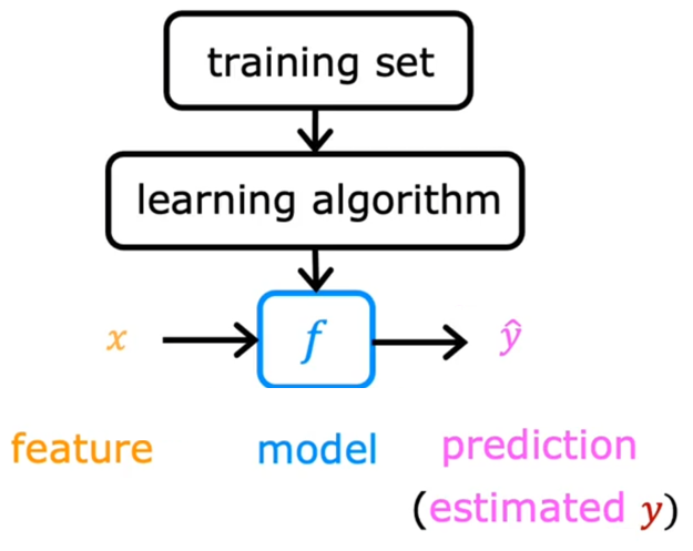
$f$ is the function or model getting from the learning algorithm, which can be used to predict the output. $\widehat{y}$, the value of $f$, is the prediction of $y$.

Linear regression model

Linear regression model is the most simple model in regression model, in which, $f$ is just a linear function:

$${f}_{w,b}(x)=wx+b$$

or

$$f(x)=wx+b$$

$w$ and $b$ are the parameters that we (the learning algorithms) can adjust to make $f$ more accurate.

Linear regression with single input is also called univariate linear regression.

Cost function

Cost function compares $\widehat{y}$ to $y$. The better the model is, the smaller the value of the cost function is. The simplest and most commonly used cost function in linear regression is:

$$J_{(w,b)}=\frac{1}{2m}\sum\limits_{i=1}^{m}(\widehat{y}^{(i)}-y^{(i)})^2$$

which is called mean squared error cost function.

Why $2m$?

This is for the convenience of later calculations. When deriving $J$ using the gradient descent method, if it is $2m$, there will not be any constant in the derivative function:

$$\frac{\partial{J_{(w,b)}}}{\partial{w}}=\frac{1}{m}\sum\limits_{i=1}^{m}(\widehat{y}^{(i)}-y^{(i)})\frac{\partial{\widehat{y}^{(i)}}}{\partial{w}}$$

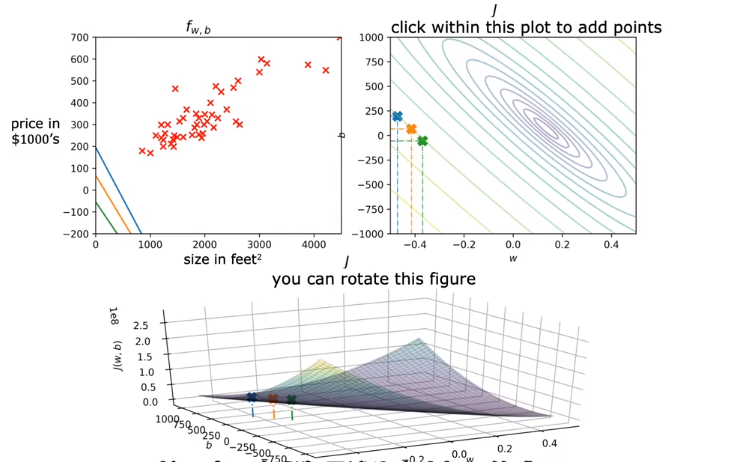
Since the training set is constant, $J$ is just the function of $w$ and $b$. Therefore, our goal is to find $w$ and $b$ that minimize $J_{(w,b)}$.

The 3D bowl-shaped surface plot, which is the plot of $J$, can also be visualized as a contour plot. In the contour plot, each oval contains the choices of $w$ and $b$ that result in the same value of $J$.

Fig. 2. 3D plot and contour plot

Gradient descent

Gradient descent is an algorithm that can be used to minimize any function. The steps of gradient descent are:

1. Start with some parameters (just set them to 0 is ok);

2. Keep changing the parameters to reduce $J$:
   $$w=w-\alpha\frac{\partial{J_{(w,b)}}}{\partial{w}}$$
   $\alpha$: learning rate, (0,1], which is used to control the speed of gradient descent.

   $w$: any parameter.

   All the parameters should be updated simultaneously, which means that when updating one parameter, the value of other parameters should be their original values.

   Principle: The ${grad(f)}$ at a certain point is the direction in which the function changes the fastest.

3. Get a minimum or near minimum $J$.

To achieve this, $J$ has to be a bowl shape function (convex function) or a function with local minima.

Fig. 3. Function with locak minima

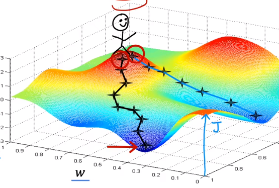
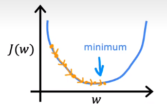
In linear regression, mean squared error cost function is always a bowl shape function because it squares the loss. If $\alpha$ is too small, the gradient descent will work but may be very slow.

Fig. 4. Model with small learning rate

If $\alpha$ is too large, the gradient descent may not work, which means it may fail to converge but diverge.

Fig. 5. Model with large learning rate

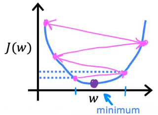
Batch gradient descent: Each step of gradient descent uses all the training examples.

Multiple linear regression model

When there are more than one features determining the output, it is advisable for us to use vector.

Feature engineering: Using intuition to design new features by transforming or combining original features. Good features will make the model better.

Notation

• $x_j$ = $j^{th}$ feature;
• $n$ = number of features;
• ${\vec{x}^{(i)}}$ = features of $i^{th}$ training example.
• $x_j^{(i)}$ = value of feature $j$ in $i^{th}$ training example ($x$ can also be $\vec{x}$).

Model

$$f_{w,b}(x_1,x_2,...,x_n)=w_1x_1+w_2x_2+...+w_nx_n+b$$

is equal to:

$$f_{\vec{w},b}(\vec{x})=\vec{w}\cdot\vec{x}+b$$

where

$$\vec{w}=[w_1,w_2,...,w_n],\vec{x}=[x_1,x_2,...,x_n]$$

Vectorization

import numpy as np
w = np.array([1.0, 2.5, -3.3])
b = 4
x = np.array([10, 20, 30])
# vectorization
f = np.dot(w, x) + b

np.dot() can make use of parallel hardwares, so it is much faster than for loop. (SIMD)

GPU will help to deal with vectorized code.

Cost function

The cost function can also be represented as $J(\vec{w},b)$. All the parameters $\vec{w}$ and $b$ should also be updated simultaneously.

Normal equation: This method only works for linear regression. It sovles for $w,b$ without iterations. However, it does not generalize to other learning algorithms and it is slow when the number of features is too large (>10,000). It may be useful on the backend.

More about gradient descent

Feature scaling

Feature scaling is a mothod to accelerate gradient descent. When the value of some features is too large, what may happen is that even though $\alpha$ is small, the changes of some parameters are still too significant, which slows down the convergence speed of gradient descent.

Fig. 6. Unscaled features

One useful method is feature scaling. By scaling down some features, we can make the convergence speed of different parameters basically the same.

Fig. 7. Scaled features

Ways to scale features:

• Dividing by the maximum of the feature;
• Mean normalization. This method may produce negative value, but the range of feature is always 1.To realize this:
  1. Get the mean value of this feature in the training set $\mu$;
  2. Subtract $\mu$ from each example of this feature and divide the result by the difference between the maximum and minimum values of this feature.
     $$x=\frac{x-\mu}{max-min}$$
• Z-score normalization. $\sigma$ is the standard deviation of this feature.
  $$x=\frac{x-\mu}{\sigma}$$

  When predicting, the new $x$ should also be scaled using the same parameters as before.

Ways to check convergence

1. Draw $J-iterations$ curve or learning curve.

Fig. 8. Iterations curve

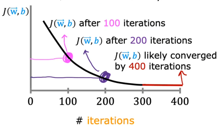
2. Automatic convergence test: Let $\epsilon$ be a small value. Once $J$ decreases by $\leqslant$ $\epsilon$ in one iteration, it converges.

Choose a better $\alpha$

Once the learning curve looks like these:

Fig. 9. Model with large learning rate

It indicates that $\alpha$ is too large. The way to choose a good $\alpha$ is starting with a relative small value (like 0.001). And check the astringency of $J$. If $J$ still does not converge, there may be some bugs in the code. Then, we can try to increase $\alpha$ by three times, until we find a relative large $\alpha$.

Polynomial regression

In polynomial regression, the model $f$ is a polynomial, which means that one feature may occur several times with different powers. For example:

$$f(x)=w_1x+w_2\sqrt{x}+b$$

In fact, by changing the power, one feature can produce infinite features. That is, $x$ and $\sqrt{x}$ are two different features.

Since they are actually different features, we can use another variable to represent them. Then, the function may become: $f(x,z)=w_1x+w_2z+b$. It is a linear function formally.

Compared to linear regression, in polynomial regression, feature scaling and the selection of feature are more important.

Classification model

Binary classification model

When the output of classification model only has two possible values, such classification model can also be named binary classification. In binary classification, we always use 0 (false) and 1 (true) to represent the output. 0 is also called negative class and 1 is also called positive class.

Logistic regression is the most commonly used model in binary classification:

$$f_{(\vec{w},b)}{(\vec{x})}=g(\vec{w}\cdot\vec{x}+b)=g(z)=\frac{1}{1+e^{-(\vec{w}\cdot\vec{x}+b)}}$$

where

$$g(z)=\frac{1}{1+e^{-z}},0<g(z)<1$$

is called sigmoid function or logistic function.

Fig. 10. Sigmoid function

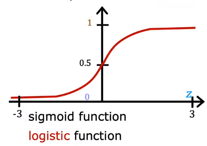
Actually, the output of logistic regression can also be regarded as the possibility of y==1, so $f$ can also be represented as:
$$f_{(\vec{w},b)}{(\vec{x})}=P(y=1|\vec{x};\vec{w},b)$$

Decision boundary

Since the output of logistic regression should be either 0 or 1, we must turn the value between 0 and 1 to 0 or 1. That is, we should find a threshold. When $f \ge threshold$,$f=1$, otherwise, $f=0$. The threshold we choose is often 0.5. When $f \ge 0.5$ ($\widehat{y}=1$):
$$g(z) \ge 0.5$$
$$\downarrow$$
$$z \ge 0$$
$$\downarrow$$
$$\vec{w}\cdot\vec{x}+b \ge 0$$
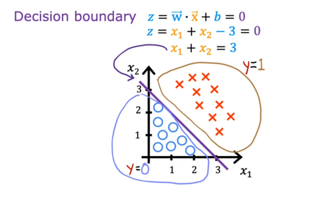
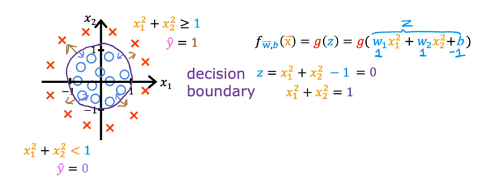
The curve $\vec{w}\cdot\vec{x}+b = 0$ is called decision boundary, where $\widehat{y}$ could be 0 or 1. For example:

Fig. 11. Decision boundary-line

Fig. 12. Decision boundary-circle

Loss function

In linear regression, the cost function:

$$J_{(w,b)}=\frac{1}{2m}\sum\limits_{i=1}^{m}(f_{\vec{w},b}(\vec{x}^{(i)})-y^{(i)})^2$$

can also be represented as:

$$J_{(w,b)}=\frac{1}{m}\sum\limits_{i=1}^{m}\frac{1}{2}(f_{\vec{w},b}(\vec{x}^{(i)})-y^{(i)})^2$$

where:

$$L(f_{\vec{w},b}(\vec{x}^{(i)}),y^{(i)})=\frac{1}{2}(f_{\vec{w},b}(\vec{x}^{(i)})-y^{(i)})^2$$

is called loss function.

Loss function indicates the error between the prediction value and real value of one example in training set. The convexity of cost function is actually determined by loss function. In logistic regression, squared error loss function is a non-convex function.

Fig. 13. Non-convex loss function

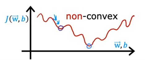
Therefore, a new convex function is needed in logistic regression, that is:
$$L(f_{\vec{w},b}(\vec{x}^{(i)}),y^{(i)})=-y^{(i)}\log(f_{\vec{w},b}(\vec{x}^{(i)}))-(1-y^{(i)})\log(1-f_{\vec{w},b}(\vec{x}^{(i)}))$$
where $y^{(i)}=0,1$; $f_{\vec{w},b}(\vec{x}^{(i)})\in(0,1)$; $\log$ uses $\ln$.

When $y^{(i)}=1$, the curve of $L$ is:

Fig. 14.

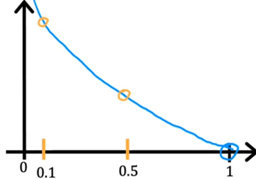
Using gradient descent will make the loss close to 0.

When $y^{(i)}=0$,the curve of $L$ is:

Fig. 15.

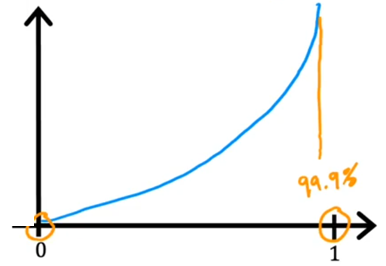
Using gradient descent will also make the loss close to 0.

Cost function

$$J_{(w,b)}=-\frac{1}{m}\sum\limits_{i=1}^{m}[y^{(i)}\log(f_{\vec{w},b}(\vec{x}^{(i)}))+(1-y^{(i)})\log(1-f_{\vec{w},b}(\vec{x}^{(i)}))]$$
The derivative of $J$ in logistic regression is actually the same as that in linear regression:
$$w_j=w_j-\alpha[\frac{1}{m}\sum\limits_{i=1}^{m}(f_{\vec{w},b}(\vec{x}^{(i)})-y^{(i)})x_j^{(i)}]$$
$$b=b-\alpha[\frac{1}{m}\sum\limits_{i=1}^{m}(f_{\vec{w},b}(\vec{x}^{(i)})-y^{(i)})]$$

However, the model $f$ is different.

Vectorization and feature scaling can also be used in losgistic regression.

Multiclass classification model

See Softmax regression.

Multi-layer classification model

See Multi-label classification.

Regularization

Underfitting

When a model does not fit the training set well, the model is underfitting,

Fig. 16. Underfitting model

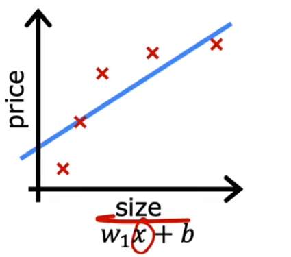
An underfitting model is an algorithm having high bias. In this case, we need to change a model.

Overfitting

When a model fits the training set extremely well, that is, the errors are approximate 0, the model is overfitting.

Fig. 17. Overfitting model

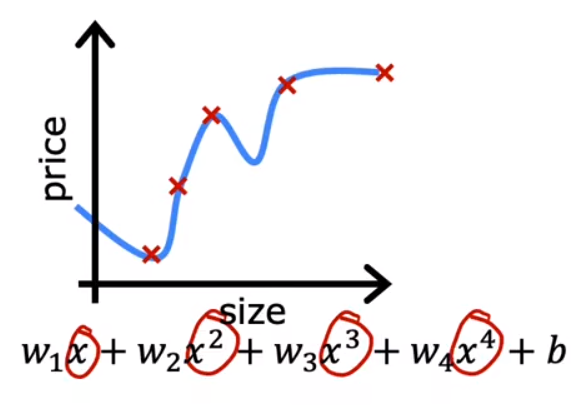
An overfitting model is an algorithm having high variance. In this case, the model just fits the training set well, but it can not be generalized. This problem often occurs when the training set is too small. So, the first method to solve this problem is to collect more training examples. Besides, selecting more suitable features is also feasible (Feature Selection). However, this method may cause our model to lose some useful features. The most feasible and commonly used method is regularization.

Weight decay

Overfitting may occurs when some features have an overly large effect, that is, a little change of these features may cause large changes to the model, which can make the model unexpandable.

The core idea of regularization is to reduce the weight of features with large value. When regularizing, the cost function $J$ becomes:

$$J(\vec{w},b)=\frac{1}{m}\sum\limits_{i=1}^{m}L(f_{\vec{w},b}(\vec{x}^{(i)}),y^{(i)})+\frac{\lambda}{2m}\sum\limits_{j=1}^{n}w_j^2$$

We just need to regularize $w_j$ as $b$ just makes $f$ move up or down.

$\lambda$ (>0) is an important parameter that balance fitting data and keeping $w_j$ small. In fact, this is Lagrange multiplier, a method to find local extremea of a multivariate function when its variables are constrained by one or more conditions. The restriction here is $\frac{1}{2m}\sum\limits_{j=1}^{n}w_j^2=0$. Since we have limited the value of $\lambda$, our function doesn't obey the constraint strictly but the constraint does make $w$ smaller and the curve more smooth.

Since $J$ changes, the update of $w_j$ will also change:

$$w_j=w_j-\alpha[\frac{1}{m}\sum\limits_{i=1}^{m}\frac{\partial{L(f_{\vec{w},b}(\vec{x}^{(i)}),y^{(i)})}}{\partial{w_j}}+\frac{\lambda}{m}w_j]$$
or
$$w_j=(1-\alpha\frac{\lambda}{m})w_j-\alpha\frac{1}{m}\sum\limits_{i=1}^{m}\frac{\partial{L(f_{\vec{w},b}(\vec{x}^{(i)}),y^{(i)})}}{\partial{w_j}}$$

The second formula indicates that in each iteration, $w_j$ will be smaller than before. Therefore, this kind of normalization is also called weight decay.