Tensorflow
Basic data structure
See Numpy and Tensorflow.
Neural networks
Normalize data
Fitting the weights (w, b) to the data will proceed more quickly if the data is normalized. In tensorflow, we can use Normalization to normalize data. It uses z-score. However, it is a preprocessing layer rather than an independent layer of model.
1 | from tensorflow.keras.layers import Normalization |
axis=-1means that it will normalize the last dimension ofX. For 2-D arrays, it will normalize the column. In this case,axis=-1is equal toaxis=1.- After normalizing, the test set should also be normalized:
X_testn = norm_l(X_test).
Create the model
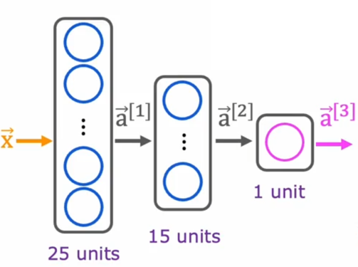
For a neural network like this:

we can create the neural network using tensorflow in Python:
1 | import tensorflow as tf |
Keras is an open-source software library that provides a Python interface for neural networks. It is now a package under tensorflow,which acts as an interface.
unitsrepresents the number of neuron in this layerr.activationrepresents theactivation functionyou choose for this layer.Denseis a kind of hidden layer that make use of all the inputs for each neuron.- We can also assign names to each layer using
name='xx'. For the first layer, usinginput_dim=xxis another way to specify the shape of input layer.- When specifying the shape of input layer,
modelwill be instantiated. That is, parameters of all layers will be initialized.- Use
.summaryto get the structure of model. Use.get_layer('layer_name')to get the certain layer.
We can also create the neural network layer by layer:
1 | import numpy as np |
For each layer, we can use
.get_weights()to get itswandb. Feed some examples to instantiate them or use.set_weights([w, b])to initialize them.
The first way is more convenient and universal, as it builds a neural network at once.
Name of activation functions in keras:
- relu
- sigmoid
- linear
- softmax
- ...
Loss and cost functions
1 | from tensorflow.keras import losses |
See Adam algorithm to know more about Adam.
At this step, the structure of the neural network has already been established.
The name of some loss functions in
losses:
- BinaryCrossentropy: Binary classification
- MeanSquaredError: Linear regression
- SparseCategoricalCrossentropy: Multiclass classification
If we regard the whole neural network as a generalized model, the model and cost function can be represent as:
$$
f(W,B)(\vec{x})
$$
$$
J(W,B)=\frac{1}{m}\sum\limits_{i=1}^{m}L(f(\vec{x}^{(i)},y^{(i)}))
$$
Regularization
When regularization, we just need to add:
1 | kernel_regularizer=tf.keras.regularizers.l2(0.1) # 0.1 is the value of lambda |
to the layer that we want to regularize.
Gradient descent
This is the final step to train a neural network. In this step, we use gradient descent to determine $W$ and $B$.
Capital means matrix
1 | model.fit(X, y, epochs=100) |
The algorithm used in fit is called Backpropagation. X,y is our training set and epochs represents the number of iterations.
After finishing the training of neural network, we can use model.predict() or model() to predict or infer.
The type of
model.predict()istfwhile the type ofmodel()isnp.
Optimization for softmax
In multiclass classfication, the following code will work, but the value is not very accurate. See Softmax regression to know more about multiclass classification and softmax.
1 | import tensorflow as tf |
Due to the limitations in precision when using binary to represent decimals, the more intermediate values we use, the greater the loss of precision we get. Before we calculate $loss$, we must get the value of $a$. $a$ is a intermediate value, so it is advisable for us to replace $a$ in $loss$ with its original formula. That is:
$$a_i=g(z)=\frac{e^{z_i}}{e^{z_1}+...+e^{z_i}}$$
$$loss=-\log{a_1}, y=1...$$
$$\downarrow$$
$$loss=-\log\frac{e^{z_i}}{e^{z_1}+...+e^{z_i}},y=1...$$
To realize this, we just need to set the activation function of output layer to linear and set from_logits to True:
1 | model = Sequential([ |
The principle of this code is that $g(z)$ is just $z$, and tensorflow will replace $a$ with its original formula in loss function. from_logits actuallly means use $z$ rather than $a$. This gives tensorflow more flexibility to rearrange the terms to get more accurate values.
In this case, the output of our neural network is actually a vector of $z$. Therefore, we have to add
2
f_x = tf.nn.softmax(logit)to get the real values. However, to get the label, we just need to use
np.argmax(y_pred, axis=0).
The same optimization can also be applied to other neural networks, like binary classification.
Regression model
For regression models, Auto Diff (Auto Grad) of Tensorflow can help us get partial derivatives automatically.
Gradient descent
1 | import tensorflow as tf |
Adam algorithm
The example used here is about collaborative filtering. See Collaborative filtering to know more about it.
1 | from tensorflow import keras |