Machine Learning Diagnostics

Evaluating a model

To evaluate a model is to measure the accuracy of the model's predictions. There are many ways to do so.

Two sets

One useful method is to splite our training set into training set and test set. Training set is used to train and evaluate the model, but test set is only applied to evaluate the model. To evaluate a trained model, we should calculate both the $J_{test}$ and $J_{train}$, both of which are without regularization term. But the model is regularized.

For classification model, we can also count the number of misclassified examples in training set and test set respectively.

Choosing a model

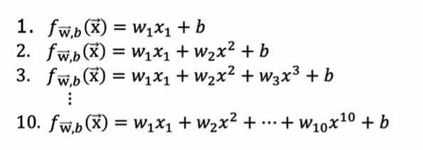
To choose a model or to determine the architecture of a model, using two datasets suffers from the same problems as evaluating models on one dataset.

When evaluating a model on one dataset, we actually get an optimistic estimate of generalization error. That is, the model only fits the training set well but can not be generalized. The same problem will happen when choosing a model with two datasets. When we use the test set to choose a model, it is likely that the model may just fit this test set well as the structure of the model is also a parameter like $W$ and $B$. In conclusion, we can not use datasets that determine the model to evaluate or choose a model.

Fig. 1. Model choosing

Three sets

The solution is to divide the dataset into three parts: training set, cross validation set and test set.

Cross validation set is also called development set or dev set.

The procedure of choosing a model is similar to evaluating a model:

• Train the model using training set, get $W$ and $B$;
• Choose a model using development set, calculate $J_{cv}$ and get d (degree of polynomial);
• Verify the model using test set, calculate $J_{test}$.

type	training set	dev set	test set
trained	yes	no	no
function	get $W$ and $B$	determine model structure	evaluate generalization ability of model
usage count	multiple times	multiple times	one time

A vivid metaphor about these sets is: Training set is students'textbook, dev set is students'homework and test set is the final exam.

Diagnostics

Bias and variance

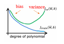
Instead of plotting the model to judge underfitting or overfitting, a more common method is to calculate and compare $J_{train}$ and $J_{cv}$.

• If $J_{train}$ is high and $J_{train}\approx J_{cv}$, the algorithm(model) may have high bias;
• If $J_{train}$ is low and $J_{train}<<J_{cv}$, the algorithm(model) may have high variance;
• If $J_{train}$ is high and $J_{train}<<J_{cv}$, the algorithm(model) may have high bias and high variance.

  An algorithm having both high bias and high variance fits some training examples well but fits others badly.

Fig. 2. Relationship between D and error

Choosing a good $\lambda$

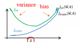
We can also use the dev set to choose a better regularization parameter $\lambda$.

• If $\lambda$ is rather small, we value fitting the data. Therefore, $J_{cv}$ may be rather high while $J_{train}$ may be rather low;
• If $\lambda$ is rather big, we value scaling $\vec{w}$. Therefore, $\vec{w}$ is aproximate 0, $J_{cv}$ may be rather high and $J_{train}$ may also be rather high.

Fig. 3. Relationship between lambda and error

Quantitative indicators

In order to judge bias or variance quantitatively, a baseline level of performance is required. It can be human level performance, competing algorithms performance or just guess based on experience.

• When gap between baseline and $J_{train}$ is rather high, the model may have high bias;
• When gap between $J_{train}$ and $J_{cv}$ is rather high, the model may have high variance.

Learning curve

Learning curve is a function curve of training set size and error of training set and dev set. We can use learning curve to judge whether a model has high bias or high variance. A regular learning curve looks like:

Fig. 4. Regular learning curve

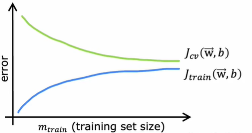
When a model has high bias, its learning curve looks like:

Fig. 5. High bias learning curve

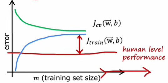
It indicates that when a model has high bias, we can not train a good model by using more data.

When a model has high variance, its learning curve looks like:

Fig. 6. High variance learning curve

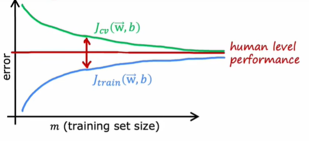
It indicates that when a model has high variance, we can train a better model by using more data because your model is complicated enough. Though learning curve gives us an intuitive visual experience of the performance of our model, it is seldom used as plotting it wastes too much time.

Fixing bias variance

High variance:

• Get more training examples;
• Try smaller sets of features;
• Try increasing $\lambda$.

High bias:

• Try getting additional features;
• Try adding polynomial features;
• Try decreasing $\lambda$.

DL and bias variance

In deep learning, the contradiction between high bias and variance can be easily solved. In general, large neural networks are low bias machines as we can reduce bias by adding more layers or neurons. For variance, we can solve it by adding more data. As long as regularization is chosen appropriately, a large neural network will usually do as well or better than a smaller one.

Fig. 7. Training of neural networks

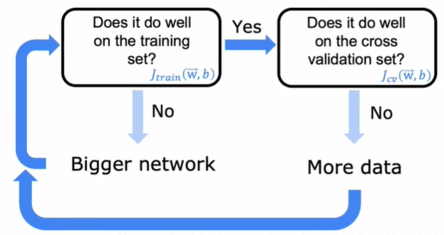
A bigger network needs powerful computing power to train. Therefore, the development of hardwares, especially GPU, and big data contribute to the thriving of deep learning.

Error analysis

Error analysis is another useful diagnostics method when training a model. In error analysis, we take the examples that the model has wrongly predicted or inferred into account and group them into common themes or common properties. These categories can be overlapping. Sometimes, the error set may be too large for us to deal with. In this case, it is advisable to randomly sample a subset (usually 100 examples).

In the next step, we can modify the model according to these categories. It is advisable to process the categories that are large enough but just ignore those small categories.

Skewed datasets

Skewed datasets are datasets that have an uneven subset distribution. That is, the number of one output is much more than the others. In this case, we can't simply judge the performance of model using $J$ as we may get a good result even if the model just predicts this label all the time.

The solution is to count precision and recall of the model. In binary regression (for multiclass classfication, we set the real label 1 and the others 0), we can display the true value and predict value in the form of 2*2 matrix:

Fig. 8. Output distribution

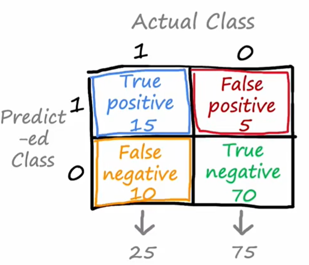
Then precision is defined as the fraction that are actually 1 among all examples where we predicted $y=1$:
$${Precision}=\frac{TruePos}{TruePos+FalsePos}$$

Recall is defined as the fraction that are correctly predicted among all examples that are actually 1:
$${Recall}=\frac{TruePos}{TruePos+FalseNeg}$$

A good model should have both high precision and recall. Once precision or recall is 0, chances are that the model print("y=0") all the time.

$F_1 score$: Trading off precision and recall

For logistic regression, threshold is the boundary value used to separate 0 and 1. If raising the threshold, we will get higher precision but lower recall. If decreasing the threshold, we will get higher recall but lower precision. We can't keep both precision and recall high. What's more, we can't solve this problem using dev set as threshold is defined by us.

Fig. 9. Precision and recall

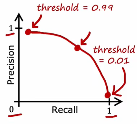
The method to compare precision and recall is to calculate $F_1 \space score$:
$$F_1\space{score}=\frac{1}{\frac{1}{2}(\frac{1}{P}+\frac{1}{R})}=\frac{2PR}{P+R}$$

The larger the $F_1 \space score$ is , the better the model is.

ROC & AUC

$F_1 \space score$ requires us to choose a threshold to judge the performance of the classifier while ROC and AUC are more intelligent.

Receiver operating characteristic curve (ROC) is a curve whose $x$ axis is False positive rate (FPR) and $y$ axis is True positive rate (TPR)：

$$
\begin{align*}
TPR=Recall&=\frac{TruePos}{TruePos+FalseNeg}\\
FPR=&\frac{FalsePos}{FalsePos+TrueNeg}
\end{align*}
$$

Fig. 10. ROC

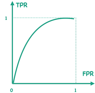
Each point on ROC represent a $(FPR, TPR)$ pair under a certain threshold. For example:

• If threshold is 0, all the samples will be predicted as 1. In this case, both FPR and TPR is 1;
• If threshold is 1, all the samples will be predicted as 0. In this case, both FPR and TPR is 0;
• With threshold decreasing, points on ROC moves to the top right (or right/or up), or remains stationary;
• When points on ROC are on $y=x$, the classifier has no difference with random guesses. The closer the points are to the upper left corner, the better the classifier is;
• Points on ROC should always be above $y=x$ as when points on ROC are below $y=x$, just letting the classifier make the opposite conclusion will make these points on top of $y=x$.

Area under curve (AUC) is the area below ROC. If we randomly pick a positive sample and a negative sample, AUC represents the probability that the classifier predicts the value of the positive sample is bigger than the value of the negative sample. Taking AUC as an indicator to measure the performance of a classifier helps us dismiss the influence of skewed datasets and threshold. In other words, AUC measures the ability of the classifier to correctly sort samples. That's why AUC is a more commonly used indicator.

Since we can't take all the values of threshold into account, we can only use the approximate method to calculate AUC, that is, computing the rate that the value of the positive sample is bigger than the value of the negative sample among all the postive-negative pairs. For a dataset with $M$ positive sample and $N$ negative samples, the number of positive-negative pairs is $M\times N$:

1. Sort the values of all the positive and negative samples from largest to smallest;
2. Score them from $N+M$ to $1$;
3. Sum the score of positive samples;
4. Subtract $M(M+1)/2$;
5. Divide by $M\times N$:
   $$AUC=\frac{\sum _{i\in\text{positive}}\text{score}_i-M(M+1)/2}{MN}\tag{1}$$

Such a process works as $\text{score} _i$ is the score of the $i$-th biggest positive sample ($i=1,...,M$) and

$$
N+M-\text{score}_i-(i-1)
$$

is the number of negative samples whose score is higher than it. Then

$$
\begin{align*}
N-[N+M-\text{score}_i-(i-1)]
&=\text{score}_i+(i-1)-M\\
&=\text{score}_i-(M+1-i)
\end{align*}
$$

is the number of positive-negative pairs that consist of the $i$-th positive sample and negative samples whose values are smaller than the positive sample. As a result, the number of positive-negative pairs that meet our requirement is

$$
\sum\limits _{i=1} ^{M}[\text{score}_i-(M+1-i)]=\sum _{i\in\text{positive}}\text{score}_i-M(M+1)/2
$$

In sklearn, function sklearn.metrics.roc_auc_score could calculate the AUC of a classifier.

From the relationship between AUC and threshold, it can be seen that: if a large threshold is used in actual deployment, a little FP can bring us large TP. As a result, the precision of the classifier will be very high. Since it is not necessary to classify all positive classes, using different threshold in training and deployment is quite reasonable.