Unsupervised Learning

Clustering

Clustering is a type of unsupervised learning that automatically groups a set of objects in such a way that objects in the same group are more similar to each other than to those in other groups. A commonly used algorithm of clustering is K-means algorithm.

K-means algorithm

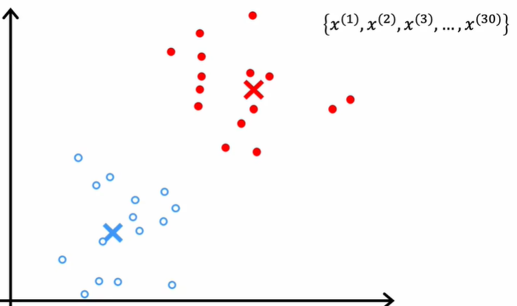
K-means algorithm partition $n$ observations into $k$ clusters where each observation belongs to the cluster with the nearest mean. In other words, there is a centroid in each cluster and among all the centroids, an observation in its cluster is closer to its centroid than to other centroids, that is, observations in the same cluster are more related. The procedures of k-means are as follows:

Cluster centroids: centers of cluster.

• Randomly initialize $K$ cluster centroids $\mu_1,\mu_2,..., \mu_K$;

  Just randomly choose $K$ points from the training set is ok though different initialization will produce different clusters.

• Assign points to its closest cluster centroids;

  If there are no points assigned to a centroid, just reduce the number of centroids to $K-1$ or reinitialize the centroids.

• Move each cluster centroid to the average of all the points $(\bar{x},\bar{y},..., \bar{z})$ that were assigned to it;
• Keep doing so until the movements of centroids are small enough;
• Reinitialize all the centroids and train another set of $\mu$ 50-1000 times, choose the set with the lowest $J$ as the final result of clustering.

Fig. 1. K-means

Cost function

Definition of some notations:

• $c^{(i)}$ = index of cluster (1, 2,..., $K$) where example $x^{(i)}$ is currently assigned;
• $\mu_k$ = cluster centroid $k$;
• $\mu_{c^{(i)}}$ = cluster centroid of cluster to which $x^{(i)}$ has been assigned

Distortion cost function $J$:
$$J(c^{(1)},...,c^{(m)},\mu_1,...,\mu_k)=\frac{1}{m}\sum\limits_{i=1}^{m}(x^{(i)}-\mu_{c^{(i)}})^2$$

The way to minimize $J$ is repeatedly moving $\mu_k$ to the centre of cluster $k$.

Choosing a $K$

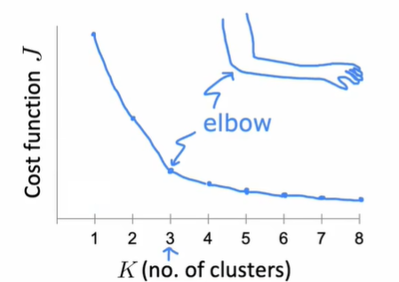
Elbow method: Choose the value at the elbow of $J-K$ curve as $K$ on elbow is the position where the slope of a function rapidly decreases.

Fig. 2. Elbow method

More generally, the choice of $K$ depends on the downstream purpose.

Anomaly detection

Anomaly detection is another type of unsupervised learning that automatically identifies rare or anomalous events which are suspicous or harmful because they differ significantly from standard behaviors or patterns. The key algorithm in anomaly detection is density estimation that builds the model of $p(x)$ which is the probability density of $x$. The most commonly used probability density model is Gaussian (Normal or Bell shaped) distribution:
$$p(x)=\frac{1}{\sqrt{2\pi}\sigma}e^{-\frac{(x-\mu)^2}{2\sigma^2}}$$

For multiple features $\vec{x}$, assuming features are independent of each other:
$$p(\vec{x})=\prod\limits_{j=1}^{n}p(x_j; \mu_j, \sigma_j^2)$$

The followings are procedures of anomaly detection:

• Choose $n$ features $x_j$ that you think might be indicative of anomalous examples;
• Fit parameters $\mu_1,...,\mu_n,\sigma_1^2,...,\sigma_n^2$;
  $$\mu_j=\frac{1}{m}\sum\limits_{i=1}^{m}x_j^{(i)}$$
  $$\sigma_j=\frac{1}{m}\sum\limits_{i=1}^{m}(x_j^{(i)}-\mu_j)^2$$
• Given new example $\vec{x}$, compute $p(\vec{x})$;
• Anomaly if $p(\vec{x})<\epsilon$.

Evaluating anomaly detection system

In anomaly detection, we actually know which example is positive and which is not, that is, we have labeled data. However, we train the model using only normal examples, cross validate model with both anomalous and normal examples to determine $\epsilon$, test model with both anomalous and normal examples. When the data set is too small, it is feasible to remove test set.

We only need to train the model one time as $\mu$ and $\sigma$ totally depend on the training set. Dev set is used to choose the best $\epsilon$. For skewed datasets, precission and recall may also be used in addition to the accurary of prediction.

Anomaly detection and supervised learning

type	Anomaly detection	Supervised learning
number of positive examples	small	large
number of negative examples	large	large
focus	detect negative examples	detect both negative and positive examples
new types of anomalies	easy to detect	hard to detect

The core idea of anomaly detection is to learn under what circumstances one example is normal. Therefore, anomaly detection is more robust if the types of anomaly keep changing while the standard of normal is stable.

Though supervised learning is also feasible when the number of positive examples is small, it can't learn much from positive examples. In contrast, since supervised learning learns what positive and negative examples look like from previous examples, it can't deal with the types of anomaly that didn't occur before well.

Choosing good features

Choosing good features is more important in anomaly detection than in supervised learning since supervised learning can rescale and take the best advantage of the features we give while anomaly detection treats each feature independent and equally important. To choose good features, there are several methods:

• Choose more gaussian features or make features more gaussian (e.g. $\log(x+c)$ instead of $x$);
  

  Fig. 3. Variable transformation
  

• Error analysis of dev set to find new features or create new features based on exsiting features.