Recommender System

Collaborative filtering

The core idea of collaborative filtering is that users tend to use items with high ratings. Therefore, by predicting users' ratings for items that they haven't used based on ratings of users who gave similar ratings, we can recommend those high rated items to users.

Notation

• $n_u$ = number of users;
• $n_m$ = number of items;
• $r(i,j)=1$ if user $j$ has rated item $i$;
• $y^{(i,j)}$ = rating given by user $j$ to item $i$;
• $w^{(j)}, b^{(j)}$ = parameters for user $j$;
• $x^{(i)}$ = feature vector for item $i$;
• $m^{(j)}$ = number of items rated by user $j$

Recommending with features

Fig. 1. Items with features

If we know the composition or features of items and their respective percentages, we can estimate how mush users like each feature or component. This is actually a regression model: ${rating}={w^{(j)}}\cdot{x}+b^{(j)}$. If we consider regularization as well as all the items and all the users together, we can get cost function $J$ like this:

$$J(w,b) = \frac{1}{2}\sum\limits_{j=1}^{n_u}\sum\limits_{i:r(i,j)=1}(w^{(j)}\cdot x^{(i)}+b^{(j)}-y^{(i,j)})^2+\frac{\lambda}{2}\sum\limits_{j=1}^{n_u}\sum\limits_{k=1}^{n}(w_k^{(j)})^2$$

It is actually a linear regression model though we only consider the items that have been rated. Since $m^{(j)}$ is different for each user and it actually doesn't affect the final result for each user because it is only related to user $j$, we can remove it and make $2m^{(j)}$ just $2$. Each user is totally independent of others, that is, $w^{(j)}$ and $b^{(j)}$ have nothing to do with others. Therefore, $J$ is just a combination of several linear regression cost functions.

Recommending without features

Fig. 2. Items without features

More generally, we don't know the exact value of each feature. Therefore, the algorithm has to learn their values from users' ratings:

$$J(x) = \frac{1}{2}\sum\limits_{i=1}^{n_m}\sum\limits_{j:r(i,j)=1}(w^{(j)}\cdot x^{(i)}+b^{(j)}-y^{(i,j)})^2+\frac{\lambda}{2}\sum\limits_{i=1}^{n_m}\sum\limits_{k=1}^{n}(x_k^{(i)})^2$$

In this case, $x$, the values of features of each item, are the parameters that the algorithm will learn. We assume that the algorithm have already known the parameters of each user. Nonetheless, it actually doesn't know. Since the first term of $J(w,b)$ and $J(x)$ are the same, we can combine them together:

$$J(w,b,x) = \frac{1}{2}\sum\limits_{(i,j):r(i,j)=1}(w^{(j)}\cdot x^{(i)}+b^{(j)}-y^{(i,j)})^2+\frac{\lambda}{2}\sum\limits_{i=1}^{n_m}\sum\limits_{k=1}^{n}(x_k^{(i)})^2+\frac{\lambda}{2}\sum\limits_{j=1}^{n_u}\sum\limits_{k=1}^{n}(w_k^{(j)})^2$$

This is collaborative filtering. In addition to learning $w$ and $b$, it also learns $x$. When gradient descent, it has to modify $w$, $b$ and $x$ simultaneously. Because of the removing of $m^{(j)}$, it can combine the first term of $J(w,b)$ and $J(x)$ together. The ratings of other users are used to learn $x$ but affect the learning of $w$ and $b$ of all the users indirectly. That's why it is called collaborative filtering - all users collaborate to generate the features of items.

If the rating of a item is given in the form of binary label (like or dislike), we can just turn linear regression to logistic regression. Namely, turn activation function from linear function to sigmoid function and turn loss function from squared error to cross entropy.

Mean normalization

If there is a new user $a$ that haven't rated any items, the prediction of its rating that the collaborative filtering algorithm makes will all be zero. Because the parameters of $a$ have nothing to do with the value of the first term of $J(w,b,x)$, regularization will make them all zero and the prediction ${rating}={w}\cdot{x}+b$ will also be zero. Intuitively, we can use the average score of each item $\mu$ to predict the rating of a new user. And that's what mean normalization does:

• Subtract ${\mu}_{j}$ from each user's rating for item $j$;
• Do collaborative filtering using normalized scores;
• Make predictions: $\widehat{y}{a}^{(i)}={w_a}\cdot{x}^{(i)}+b_a+\mu{i}$

Finding related items

Features $x^{(i)}$ of item $i$ convey something about what the item is like. Therefore, we can find items similar to this item by computing:
$$||{x}^{(k)}-{x}^{(i)}||^2$$
where ${x}^{(k)}$ and ${x}^{(i)}$ are both vectors. The smaller this value is, the more similar the two items are.

Content-based filtering

Cold start problem:

• How to rank new items that few users have rated?
• How to show something reasonable to new users who have rated few items?

Though mean normalization can solve the second problem to a certain extent, it is better to use content-based filtering to solve cold start problem.

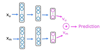
Content-based filtering recommends items to users based on features or background of user as well as item to find good match. Each user $j$ has several background information $x_u^{(j)}$ and each item $i$ has several features $x_m^{(i)}$. With $x_u^{(j)}$, it is possible for the algorithm to compute how much user $j$ like certain components of this type of item $v_u^{(j)}$. With $x_m^{(i)}$, it is possible for the algorithm to compute the proportions of each attribute of item $i$ $v_m^{(i)}$.

The dimensions of $x_u^{(j)}$ and $x_m^{(i)}$ can be different, but the dimensions of $v_u^{(j)}$ and $v_m^{(i)}$ must be the same since the prediction of rating is: $v_u^{(j)}\cdot v_m^{(i)}$.

We can use neural networks to compute $v_u^{(j)}$ and $v_m^{(i)}$ respectively:

Fig. 3. User and item network

More generally, we will combine these two neural networks together:
$$J = \sum\limits_{(i,j):r(i,j)=1}{(v_u^{(j)}\cdot v_m^{(i)}-y^{(i,j)})}^2+{regularization\space term}$$

Fig. 4. Compound neural network

The cost function of the output layer depends on the value we need. It could be mean squared error for rating or cross entropy (and sigmoid activation function) for binary result. Similarly, we can find similar items using:

$$||v_m^{(k)}-v_m^{(i)}||^2$$

Retrieval & Ranking

For one user, the algorithm only needs to count $v_u^{(j)}$ one time but it has to count $v_m^{(i)}$ for each item. If there is a large set of items, it will be time consuming. Retrieval & Ranking is one way to solve this.

In retrieval step, there is another algorithm that will generate a large list of plausible item candidates that is much smaller than the whole set.

In ranking step, the algorithm will only compute $v_m^{(i)}$ of items in the list generated in retrieval step and make recommendation.