Reinforcement Learning

Introduction

Reinforcement learning differs from supervised learning in not needing labelled input/output pairs to be presented, and in not needing sub-optimal actions to be explicitly corrected. Instead the focus is on finding a balance between exploration (of uncharted territory) and exploitation (of current knowledge).

The environment is typically stated in the form of a Markov decision process (MDP), because many reinforcement learning algorithms for this context use dynamic programming techniques. The main difference between the classical dynamic programming methods and reinforcement learning algorithms is that the latter do not assume knowledge of an exact mathematical model of the MDP and they target large MDPs where exact methods become infeasible.

wiki: Reinforcement learning

Basic concepts

• environment $E$: The environment where a agent can perceive.
• states $s$: A description of the environment perceived by a agent. It is a subset of state space $S$, that is $s\in S$.
• actions $a$: The action a agent can take. All actions form action space $A$, $a\in{A}$.
• rewards $r$: The reward a agent gets after it takes a action.
• discount factor $\gamma$: A number close to 1. It discounts the gains that require more actions and reduces the losses that require more actions.
• return: The sum of reward weighted by $\gamma$.
  $$a_1+\gamma{a_2}+...+\gamma{^n}a_{n-1}$$
• policy $\pi(s)$: A policy $a=\pi(s)$ decides the action that a agent in $s_i$ state ought to take to get to next state $s_{i+1}$ so as to maximize the return.

Fig. 1. A loop of reinforcement learning

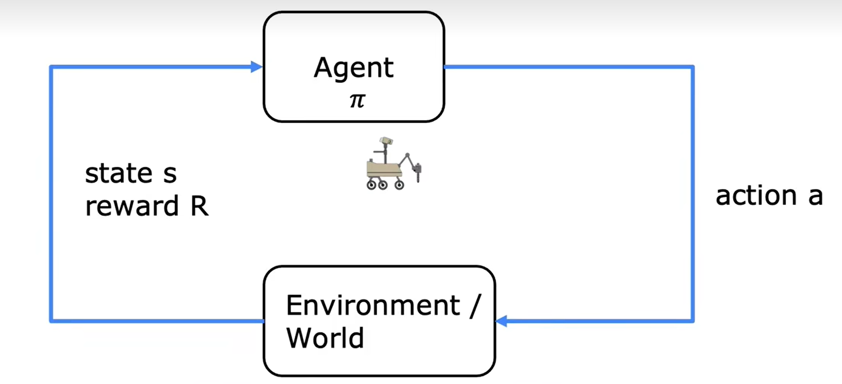
The figure above shows the procedure of reinforcement learning. A agent in state $s_i$ takes action to affect the environment or itself (The agent itself is actually a part of the environment), gets a certain reward and reach new state $s_{i+1}$. The goal of reinforcement learning is to fina a policy $\pi$ that tells the agent what action to take in every state so as to maximize the return. Nearly all reforcement learning assignment can be described as Markov decision process (MDP). MDP is a process that the future only depends on the current state $s_i$ and have nothing to do with the prior states or how things get to the current state.

State-action value function

State-action value function $Q(s,a)$, which is also called Q-function, $Q^*$ or optimal Q function, is a function that computes the maximum return a agent can get if it is in state $s$ and take action $a$ (once). After the agent takes action $a$, its state will become $s'$ and the actions it could take in state $s'$ are $a'$. It is easy to realize that the computing of $Q$ is actually a dynamic programming process. In reinforcement learning, the method we use to count $Q$ is called bellman equation:

$$Q(s,a)=R(s)+{\gamma}\max_{a'}Q(s',a')\tag{1}$$
where $R(s)$ is called immediate reward, the second part is the return weighted by $\gamma$ from behaving optimally starting from state $s'$.

Random (stochastic) environment

In practice, we can't guarantee that the agent will execute the actions precisely due to the randomness of the environment. In order to get a more precise value of return, we have to take this randomness into account:

$$
Q(s,a)=R(s)+{\gamma}E[\max_{a'}Q(s',a')]\tag{2}
$$
$E$ means expectation. When taking randomness into account, the state after taking action $a$ is uncertain. Therefore, what the second term of $Q(s,a)$ computes is the weighted average of the maximum returns weighted by $\gamma$ of the different states the agent may reach after taking action $a$.

Continuous state

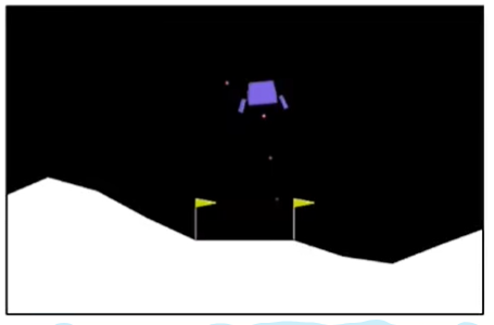
In practice, the state of a agent is a vector whose values are continuous. For examples, in lab Lunar Lander, the state of a lunar lander can be described as:
$$
s=[x,y,\dot{x},\dot{y},\theta,\dot{\theta},l,r]
$$
where $x$, $y$ and $\theta$ are its position since this is a plane problem. $\dot{x}$, $\dot{y}$, $\dot{\theta}$ are its velocity of different directions. $l$ and $r$ (value 0 or 1) indicates whether the left or right leg of lunar lander has landed.

Fig. 2. Lunar Lander

DQN algorithm

An algorithm to solve this type of reinforcement learning is DQN algorithm or Deep Q-Network. It is also called deep reinforcement learning as it uses neural networks to solve reinforcement learning problems. Its core idea is to compute $Q(s,a)$ using neural networks:

Fig. 3. Deep reinforcement learning

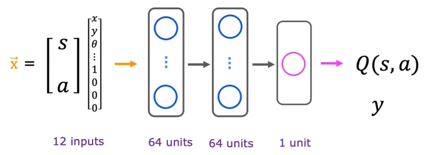
where $s$ is the state vector and $a$ is the action vector. In lunar lander, $a$ has four dimensions: do nothing, left thruster, right thruster and main thruster. Since it is actually a supervised learning model, we have to feed it training set $(s,a,Q)$ to get the mapping relationship between $s \And a$ and $Q$. According to bellman equation:

$$Q(s,a)=R(s)+{\gamma}\max_{a'}Q(s',a')$$

$Q$ is decided by $R(s)$ and $s'$ since we must take all the action $a'$ into account, that is, once we get $(s,a,R(s),s')$, we get $(s,a,Q)$. Therefore, the steps of DQN are:

1. Initialize the neural netwrok randomly as a guess of $Q(s,a)$;
2. Simulate the behaviors of the agent to get a number of $(s,a,R(s),s')$;
3. Feed $(s',a')$ to the neural network to predict $Q(s',a')$;
4. Create training set using
   $$x=(s,a) \And Q(s,a)=R(s)+{\gamma}\max_{a'}Q(s',a')$$
5. Train the neural network using training set created above, get $Q_{new}$;
6. Set $Q=Q_{new}$.

That is, produce some $(s,a,R(s),s')$ and guess a structure of $Q$ ($Q$ is the neural network). Use this $Q$ to predict $(s,a,Q)$. Use $(s,a,Q)$ to train the neural network and fine tune $Q$.

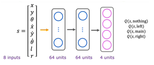
In the architecture above, for each value of $a$ in a certain state $s$, we have to predict it respectively. A more effective architecture is to just feed $s$ and produce $Q$ of all values of $a$:

Fig. 4. Improved neural network architecture

$\epsilon$-greedy policy

When simulating the behaviors of the agent, instead of simulating its action randomly, it is more advisable to choose a action that will maximizes $Q(s,a)$. However, choosing the action that maximizes $Q(s,a)$ all the time may reduce the robustness of the agent or miss some good choices. A policy to solve this is $\epsilon$-greedy policy:

• With probability $1-\epsilon$, pick the action $a$ that maximizes $Q(s,a)$;
• With probability $\epsilon$, pick an action $a$ randomly.

The first option is called 'Exploitation' and the second option is called 'Exploration'. As what the wiki in the Introduction says, reinforcement learning focuses on the balance between exploration and exploitation.

It is recommended to start $\epsilon$ high to explore more so as to enrich the robustness and then slightly reduce $\epsilon$.

Algorithm refinement

Mini-batch

When the training set is too large, it is advisable to use different subsets instead of the whole set in each iteration. This will accelerate the computation of both $J$ and derivatives. Such methods can also be used in regression model:

Fig. 5. Mini-batch

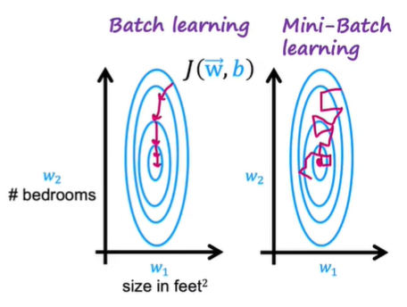
Tensorflow trains model using mini-batch.

Soft update

When updating $Q$, we can't guarantee that $Q_{new}$ is better than $Q$. Therefore, it is recommended to keep a part of $Q$ and update smoothly, like:
$$Q_{new}=0.01Q_{new}+0.99Q\tag{3}$$