D2L: Environment Configuration and Introduction

Environment configuration

Firstly, install anaconda or miniconda. Then, create a virtual environment:

conda create -n d2l-zh -y python=3.8 pip
conda actiave d2l-zh # activate the virtual environment

Install dependent packages:

pip install jupyter d2l torch torchvision

If you want to remove a virtual environment, use:

conda remove -n d2l-zh --all

Download the courseware from http://zh-v2.d2l.ai/d2l-zh.zip and unzip it. Now you can enter your conda prompt, activate virtual environment d2l-zh, enter your courseware folder d2l-zh and enter jupyter notebook to open the folder with jupyter notebook.

gym and scipy should also be installed using pip.

Introduction

This only includes what I'm interested in:

• Convolutional neural network (CNN): LeNet, AlexNet, VGG, Inception, ResNet
• Recurrent neural network (RNN): RNN, GRU, LSTM, seq2seq
• Attention mechanism: Attention, Transformet
• Optimization: SGD, Momentum, Adam
• High performance computing

Derivative of matrix

The essence of matrix derivative: Treat each element of numerator matrix as a function. Get its partial derivatives with respect to each element in denominator matrix. This is the nature of matrix derivative. However, to represent the results better, there are two most commonly used layout:

• Numerator layout: Preserve the layout of elements in the numerator $Y$. Replace each element with its derivatives with respect to denominator matrix $X^T$. This the more commonly used layout in machine learning.
• Denominator layout: Preserve the layout of elements in the denominator $X$. Replace each element with the derivatives of numerator $Y^T$ with respect to it.

The numerator layout is the transpose of the denominator layout. For examples, if the dimension of $Y$ is (m, l) and the dimension of $X$ is (n, k). Then, the dimension of $\frac{\partial{Y}}{\partial{X}}$ is (m, l, k, n) in numerator layout and (n, k, l, m) in denominator layout. Usually:

• If a vector or matrix ($\frac{\partial{Y}}{\partial{x}}$) is differentiated with respect to a scalar, the numerator layout prevails.
• If a scalar is derived from a vector or matrix ($\frac{\partial{y}}{\partial{X}}$), the denominator layout prevails.
• For vector-to-vector derivatives ($\frac{\partial{Y}}{\partial{X}}$), there are some differences, but generally based on the Jacobian matrix of the numerator layout.

Some interesting conclusions (numerator layout):

$\vec{y}$	$a$	$\vec{x}$	$A\vec{x}$	$\vec{x}^TA$
$\frac{\partial{\vec{y}}}{\partial{\vec{x}}}$	$0$	$I$	$A$	$A^T$

$A\vec{x}=(\vec{a}_1\cdot \vec{x},..., \vec{a}_n \cdot \vec{x})^T$, where $\vec{a}_i$ is the row vector of $A$

$\vec{x}^TA=(\vec{b}_1\cdot \vec{x},..., \vec{b}_n \cdot \vec{x})$ or $^T$, where $\vec{b}_j$ is the column vector of $A$

Chain rules

See Matrix derivative rules to know more about chain rules in matrix derivative. In deep learning, the result of loss function is always a scalar (the result of softmax is actually a scalar). Therefore, it is enough for us to just master the chain rules for derivative of scalar to vector and the chain rules for detivation of vector to vector (numerator layout):

1. Scalor to vector
   $$\vec{x}_1\rightarrow\vec{x}_2\rightarrow...\rightarrow\vec{x}_n\rightarrow y$$
   $$\frac{\partial{y}}{\partial\vec{x}_1}=\frac{\partial{y}}{\partial{\vec{x}_n}}\cdot...\frac{\partial{\vec{x}_2}}{\partial{\vec{x}_1}}$$
2. Vector to vector
   $$\vec{x}_1\rightarrow\vec{x}_2\rightarrow...\rightarrow\vec{x}_n\rightarrow\vec{y}$$
   $$\frac{\partial{\vec{y}}}{\partial\vec{x}_1}=\frac{\partial{\vec{y}}}{\partial{\vec{x}_n}}\cdot...\frac{\partial{\vec{x}_2}}{\partial{\vec{x}_1}}$$

It is easy to prove the correctness of these rules by evaluating the dimension of each item. To get the derivative using chain rules, there are two ways:

• Forward propagation: Calculate from $\vec{x}_2$ to $y$. T(n)=n, S(n)=1.
• Backward propagation: Calculate from $y$ to $\vec{x}_2$. T(n)=n, S(n)=n as we have to store the previous result for other parameters.

Fig. 1. Forward and backward propagation

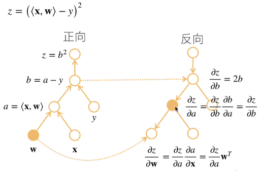
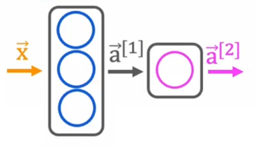
In general, backward propagation is more suitable for deep learning as it actually runs faster. In addition, a neural network can be easily represented as a computation graph as each neuron in the neural network is actually a node in computation graph:

Fig. 2. Neural network

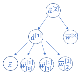
The computation graph it forms is like this:

Fig. 3. Computation graph

For convenience, we make bias=False, that is, we only compute the gradients of w. Autograd will compute gradients from $\vec{a}^{[2]}$ to the leaf nodes. That is:

$$\text{grad}[\vec{w}^{[2]}]=\frac{\partial{a^{[2]}}}{\partial{\vec w^{[2]}}}$$

$$\text{grad}[\vec{w}^{[1]}_{[i]}]=\frac{\partial{a^{[2]}}}{\partial{\vec a^{[1]}}}\cdot\frac{\partial{\vec a^{[1]}}}{\partial{\vec w^{[1]} _ {[i]}}}$$

Autograd computes from the top to bottom and store the gradients it computes before (like $\frac{\partial{a^{[2]}}}{\partial{\vec a^{[1]}}}$, autograd will store it in node $\vec a^{[1]}$) so that it doesn't need to compute it again.

Course website

• DIVE INTO DEEP LEARNING
• Course video
• autograd1
• autograd2