Attention Mechanisms: More Targeted Information Extraction

Attention in Biology

In biology, there are two kinds of cues that affect our attention: volitional cue (自主性提示) and nonvolitional cue (非自主性提示).

Fig. 1. Nonvolitional cue (left) and Volitional cue (right)

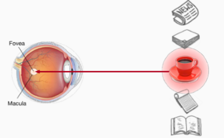
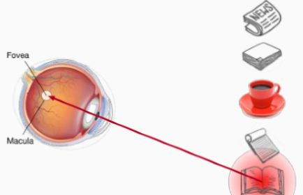
The nonvolitional cue is based on the saliency of objects in the environment. It's unconscous. As the above picture shows, when there is a red cup among several white objects, we will unconsciously choose the red cup as its color is more prominent. The volitional cue is controlled by our awareness and our decisions are led by our consciousness. For example, after drinking a cup of coffee, we may want to relax, because of which we choose a book to read.

Attention Mechanisms

The nonvolitional cue and volitional cue inspire us to take the environment as input and use volitional cue to focus the attention to a certain object or feature.

Queries, Keys and Values

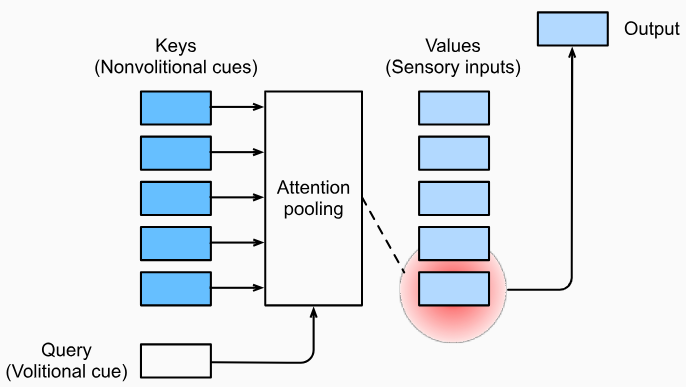
In attention mechanisms, the volitional cue is also called query. It reflects the tendency of feature extraction. The nonvolitional cue is actually our perception of the environment. The characteristics of the environment can be represented by several key-value pairs. These three things consist of the input of the attention mechanism. Giving queries and keys, the attention mechanism will aggregate values and choose the most prominent and suitable value as output. Such a process is also called attention pooling. It is queries that distinguish attention pooling from dense layers.

Fig. 2. Attention pooling

Mathematical Representation of Attention

Our attention to a certain object reflects how much we care about it, or, mathematically, the weight we give it. When a certain query is offered to us, it is natural for us to think of finding something similar to this query to get the answer. That is, for a key-value pair, the more similar the key is to the query, the higher proportion its value should take up in the answer. This is how Nadaraya-Watson kernel regression works:

$$
f(\mathbf{q})=\sum\limits _{i=1} ^n \frac{K(\mathbf{q}-\mathbf{k}_i)}{\sum\limits _{j=1} ^n K(\mathbf{q}-\mathbf{k}_j)}\mathbf{v}_i
$$

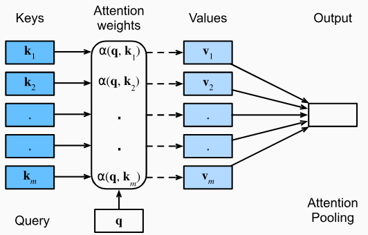
where $K$ is a kernel. Such an estimator assigns different weight to different keys for a certain query. More generally, attention is defined as:

$$
\text{Attention}(\mathbf{q},\mathbf{k},\mathbf{v})=\sum\limits _{i=1} ^n\alpha(\mathbf{q},\mathbf{k}_i)\mathbf{v}_i
$$

where $\alpha(\mathbf{q},\mathbf{k}_i)$ is attention weight. It is non-negative and its sum is $1$. The output is a weighted sum of the values for each key-value pair.

Fig. 3. Mathematical representation of attention pooling

It is noteworthy that Nadaraya-Watson kernel regression is a nonparametric model (nonparametric attention pooling). Therefore, it is consistent. With enough data, it will converge to the optimum result. However, in machine learning, the agent needs parameters to learn so that it could improve its performance. For instance, if we set $K$ as a gaussian kernel and add learned parameter $\mathbf{w}$, we get a formula that looks like softmax:

$$
\begin{align*}
K(\mathbf{u})&=\frac{1}{\sqrt{2\pi}}\exp(-\frac{\mathbf{u}^2}{2})\\
f(\mathbf{q})
&=\sum\limits _{i=1} ^n\alpha(\mathbf{q},\mathbf{k}_i)\mathbf{v}_i\\
&=\sum\limits _{i=1} ^n\frac{\exp[-\frac{1}{2}(\mathbf{q}-\mathbf{k}_i)^2\mathbf{w}^2]}{\sum\limits _{j=1} ^n\exp[-\frac{1}{2}(\mathbf{q}-\mathbf{k}_i)^2\mathbf{w}^2]}\mathbf{v}_i\\
&=\sum _{i=1} ^n\text{softmax}[-\frac{1}{2}(\mathbf{q}-\mathbf{k}_i)^2\mathbf{w}^2]\mathbf{v}_i
\end{align*}
$$

Attention Scoring Function

The exponent of the gaussian kernel above ($-{\mathbf{u}^2}/2$) is actually an attention scoring function ($a$) which evaluates the similarity between $\mathbf{q}$ and $\mathbf{k}_i$. Hence, the attention pooling can be also represented as:

$$
\begin{align*}
\text{Attention}(\mathbf{q},\mathbf{k},\mathbf{v})&=\sum\limits _{i=1} ^n\alpha(\mathbf{q},\mathbf{k}_i)\mathbf{v}_i\\
&=\sum\limits _{i=1} ^n\text{softmax}[a(\mathbf{q},\mathbf{k}_i)]\mathbf{v}_i
\end{align*}
$$

Fig. 4. Computing the output of attention pooling

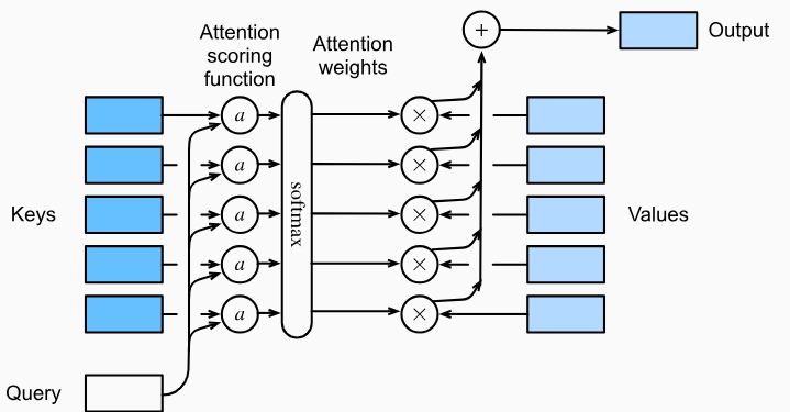
where $\text{softmax}$ generates attention weights. The more similar the key $\mathbf{k}_i$ is to the query $\mathbf{q}$, the higher weight its value $\mathbf{v}_i$ gets. The output is the weighted sum of values.

More generally, query $\mathbf{q}$ and key $\mathbf{k}_i$ are both vectors of different length. The attention scoring function maps these two vectors to a scalar

Additive Attention

Additive attention uses MLP to evaluate the similarity between $\mathbf{q}$ and $\mathbf{k}$, where $\mathbf{q}\in\mathbf{R}^q$ and $\mathbf{k}\in\mathbf{R}^k$:

$$
a(\mathbf{q,k})=[\tanh(\mathbf{q}\mathbf{W}_q+\mathbf{k}\mathbf{W}_k)]\mathbf{w}_v\in\mathbf{R}
$$

where $\mathbf{W}_q\in\mathbf{R} ^{q\times h}$, $\mathbf{W}_k\in\mathbf{R} ^{k\times h}$ and $\mathbf{w}_v\in\mathbf{R} ^{h}$. All of them are learned parameters (here we ignore the bias) in one dense layer.

In practice, each batch may have several queries and key-value pairs. And there are always more than one batches. In this case, the shape of $\mathbf{q}$ is (batch_size, num_queries, q) and the shape of $\mathbf{k}$ is (batch_size, num_kv_pairs, k). The shape of $\mathbf{q}\mathbf{W}_q$ is (batch_size, num_queries, h) and the shape of $\mathbf{k}\mathbf{W}_k$ is (batch_size, num_kv_pairs, h). num_queries and num_kv_pairs are always different, which means that we can't add $\mathbf{q}\mathbf{W}_q$ and $\mathbf{k}\mathbf{W}_k$ directly.

To solve this, we always use queries.unsqueeze(2) and keys.unsqueeze(1) (queries and keys are both tensor) to expand their dimensions. After unsqueeze, the shape of queries is (batch_size, num_queries, 1, h) and the shape of keys is (batch_size, 1, num_kv_pairs, h). Now broadcasting can make $\mathbf{q}\mathbf{W}_q+\mathbf{k}\mathbf{W}_k$ legal. The nature of this operation is that each query should take all the keys into account so the $2$-th dimension of queries is expanded to num_kv_pairs, so is keys.

Scaled Dot-Product Attention

If the shape of $\mathbf{q}$ and $\mathbf{k}$ are the same (both are $d$), we could just use dot-product to evaluate their similarity:

$$
a(\mathbf{q,k})=\mathbf{q}^\text{T}\mathbf{k}/\sqrt{d}
$$

where $\sqrt{d}$ is to make sure that the value of $a(\mathbf{q,k})$ will not change significantly when the shape changes.

If considering SGD, the output of attention pooling is:

$$
\text{softmax}(\mathbf{Q}\mathbf{K}^\text{T}/\sqrt{d})\mathbf{V}
$$

where $d$ is still the shape of each query or each key.

Different Types of Attention

Depending on the number of attention pooling and the relationship among queries, keys and values, there are various forms of attention mechanisms.

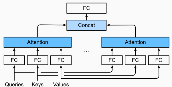
Multi-Head Attention

Just as different convolutional output channels can extract different types of features, different attention pooling will also learn various behaviors. Hence, we can use multi-head attention to generate multiple attention pooling outputs $\mathbf{h}_1...\mathbf{h}_i$ in parallel and concatenate them together to form $(\mathbf{h}_1,...,\mathbf{h}_i)$.

Fig. 5. Multi-head attention

Self-Attention

Self-attention (intra-attention) is a special kind of attention, whose queries, keys and values are all the same things.

Positional Encoding

When dealing with sequence information, RNNs operate each token in sequence. Therefore, the location information of the sequence is used. However, the attention pooling operates all the inputs in parallel, because of which, the location information is wasted.

Positional encoding is the location information added to the keys, values and queries. In computer science, we use binary string to represent position (e.g. 0: 000, 1: 001, ..., 7: 111). As can be seen, the bit on each position alternates at diferent frequencies respectively. Higher bits alternate less frequently than lower bits. Such alternating changes can represent discrete positional information.

Absolute Positional Information

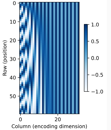
For the input $\mathbf{X}\in\mathbf{R} ^{n\times d}$ which contains $n$ tokens and $d$ features for each token, we can use positional embedding matrix $\mathbf{P}\in\mathbf{R} ^{n\times d}$ to offer it positional information:

$$
\begin{align*}
\mathbf{X'}&=\mathbf{X}+\mathbf{P}\\
\mathbf{P} _{i,2j}&=\sin(\frac{i}{10000 ^{2j/d}})\\
\mathbf{P} _{i,2j+1}&=\cos(\frac{i}{10000 ^{2j/d}})
\end{align*}
$$

It works because different columns, which are similar to the bit position in binary string, oscillate at different frequencies. It is just like the binary string but the value is continuous.

Fig. 6. Oscillating frequency of different columns

Relative Positional Information

The positional information we add to $\mathbf{X}$ is called absolute positional information. What's more, we can also get the relative positional information for different rows in the same column:

$$
\begin{align*}
(\mathbf{P} _{i,2j}, \mathbf{P} _{i,2j+1})&=(\sin\frac{i}{10000 ^{2j/d}},\cos\frac{i}{10000 ^{2j/d}})\\
(\mathbf{P} _{i+\delta,2j}, \mathbf{P} _{i+\delta,2j+1})&=(\sin\frac{i+\delta}{10000 ^{2j/d}},\cos\frac{i+\delta}{10000 ^{2j/d}})\\
&=({\begin{bmatrix}
\cos\delta\omega_j\space\space \sin\delta\omega_j\\
-\sin\delta\omega_j\space\space \cos\delta\omega_j
\end{bmatrix}}
{\begin{bmatrix}
\mathbf{P} _{i,2j}\\
\mathbf{P} _{i,2j+1}
\end{bmatrix}})^\text{T}\\
&=[\sin(i+\delta)\omega_j,\cos(i+\delta)\omega_j]\\
\end{align*}
$$

where $\omega_j=1/10000^{2j/d}$.

Positional information is information added to the input $\mathbf{X}$, including keys, values and queries, it could be fixed positional encoding like what we do above or learned one.