Diffusion

What is Diffusion Model

Sculpture is born from stone, I just cut off the part which is unnecessary. --Michelangelo

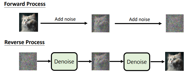
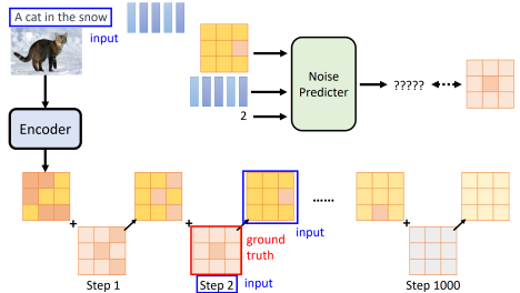
In diffusion models, while training, the 'stone' is generated from the training data by adding random noise. The sculpture is revealed by iteratively removing the noise added.

Unlike other generative models, the diffusion model does not generate data but generates noise. That is, the generator of diffusion model outputs noise, which is then removed from the noisy data. The denoised data is used as the input for the next denoising process. Therefore, the ground truth of each denoising process is the noise added and the prediction is the noise generated.

Fig. 1. Pipeline of Diffusion

Maths behind Diffusion/Generation

The goal of image generation: given $z$ from a normal distribution, output $G(z)=x$, where $x$ is similar to the original image distribution.

Fig. 2. Goal of Image Generation

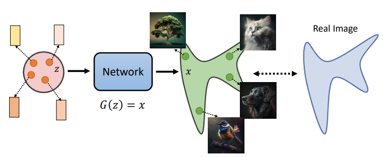
The same is true for conditional generation, except that we consider the distribution that meets this condition.

Hence, given training set $\{x^1,...,x^m\}\in P_{data}(x)$, we aim to find $\theta$ that maximizes the probability of these observations. And this is maximum likelihood estimation:

$$
\theta ^*= arg\max _\theta \prod _{i=1} ^m P _{\theta}(x ^i)
$$

Fig. 3. Maximum Likelihood Estimation (MLE)

Actually, MLE is equal to minimizing KL Divergence :

$$
\begin{align*}
\theta ^*=& arg\max _\theta \prod _{i=1} ^m P _{\theta}(x ^i)=arg\max _\theta \sum _{i=1} ^m \log P _{\theta}(x ^i)\\
\approx &arg\max _\theta E _{x\sim P _{data}} \log P _{\theta}(x)\\
=&arg\max _\theta \int _x P _{data}(x) \log P _{\theta}(x)\\
=&arg\max _\theta \int _x P _{data}(x) \log P _{\theta}(x) - \int _x P _{data}(x)\log P _{data}(x) dx\\
=&arg\max _\theta \int _x P _{data}(x) \log \frac{P _{\theta}(x)}{P _{data}(x)}\\
=&arg\min _\theta KL(P _{data}||P _{\theta})
\end{align*}
$$

Diffusion Models

Denoising Diffusion Probabilistic Models (DDPM)

In DDPM,

$$
P _\theta(x _0)=\int _{x _1:x_T}P(x _T)P _{\theta}(x _{T-1}|x _T)...P _\theta(x _{t-1}|x _t)...P _\theta(x _{0}|x _1)dx _1:x _T
$$

Fig. 4. Denoising

Similar to VAE, we actually only optimize the lower bound of $P _\theta(x)$, that is:

$$
arg\max _\theta L _b=E _{q(x _1:x _T| x)}[\log (\frac{P(x: x _T)}{q (x _1: x _T|x)})]
$$

where $q(x _1:x _T| x)=q(x _1|x)q(x _2| x _1)...q(x _T| x _{T-1})$ is the forward process, which is equal to the encoder of VAE.

Forward Process

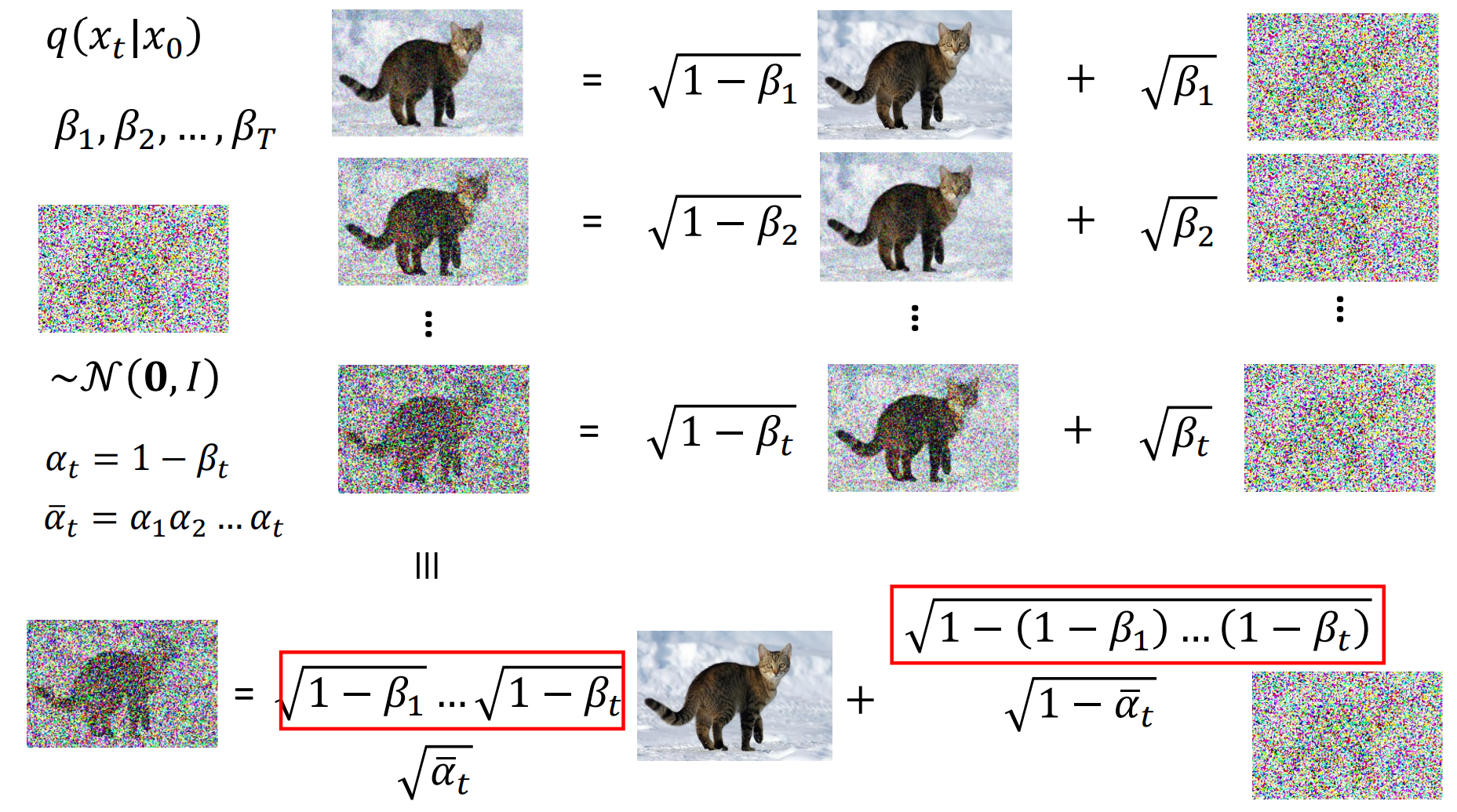
During forward process, multi-steps could be turned to single-step. As shown in the following figure:

Fig. 5. One-step Forward

Training

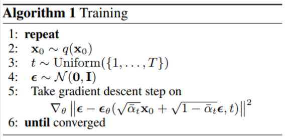
Therefore, during training, we actually only add noise once and denoise once:

Fig. 6. Training

Generation

While generating, we randomly sample data from the normal distribution and generate the image after $T$ times of denoising.

Fig. 7. Generation

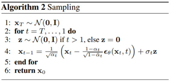
where the first term is mean and the second term is variance.

Stable Diffusion

Common architecture of modern (Text2Image) generative networks:

Fig. 8. Architecture of Modern Generative Networks

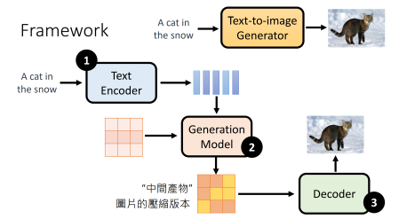
• Text Encoder: Encode text to latent representation, which is essential for the quality of final output.
• Generation Model: Any generation model, e.g., VAE, Diffusion, and GAN.
• Decoder: Decode latent representation to image.

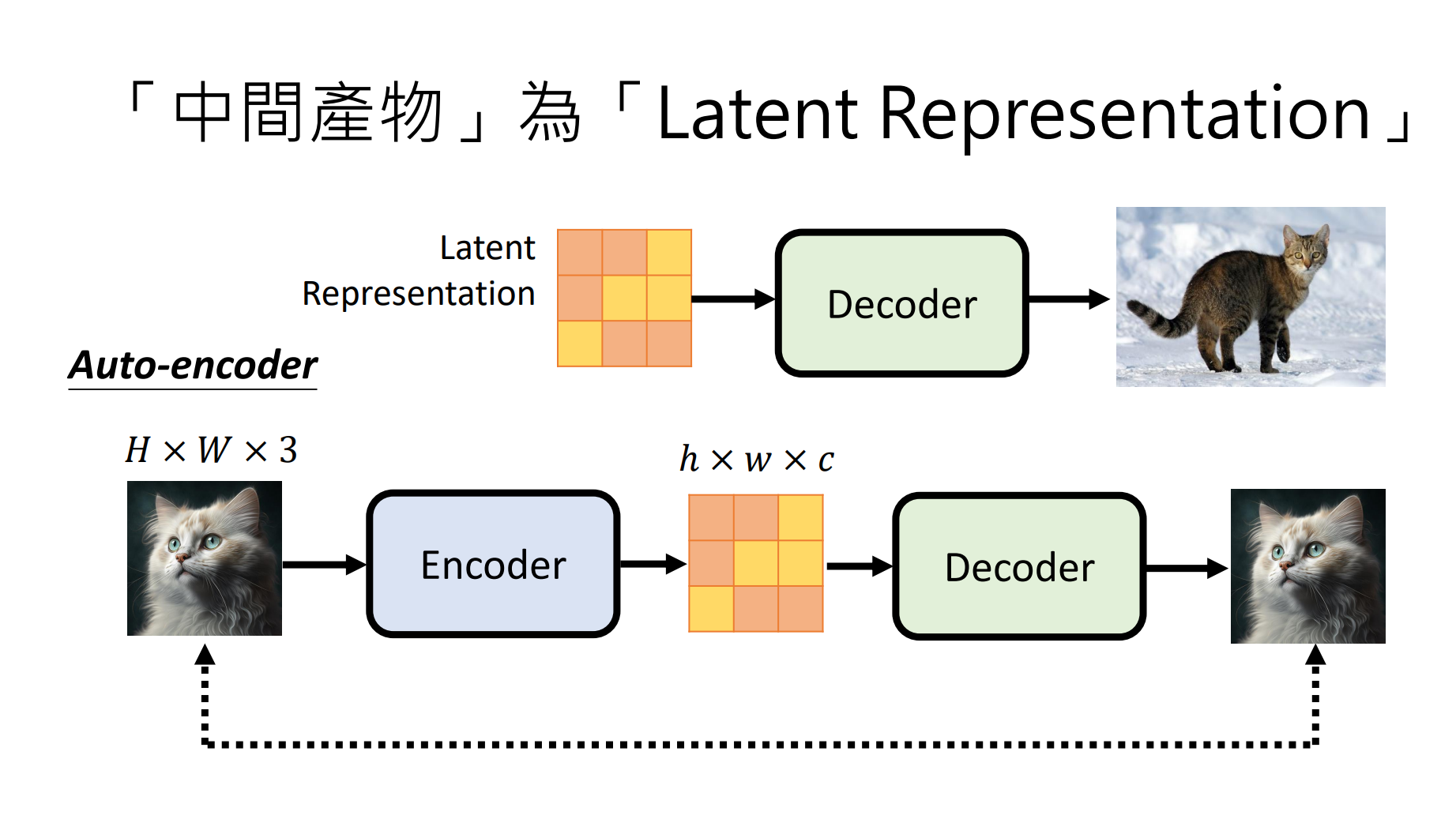
These three parts could be trained independently. For the decoder, it can accept two different inputs, depending on how you train it:

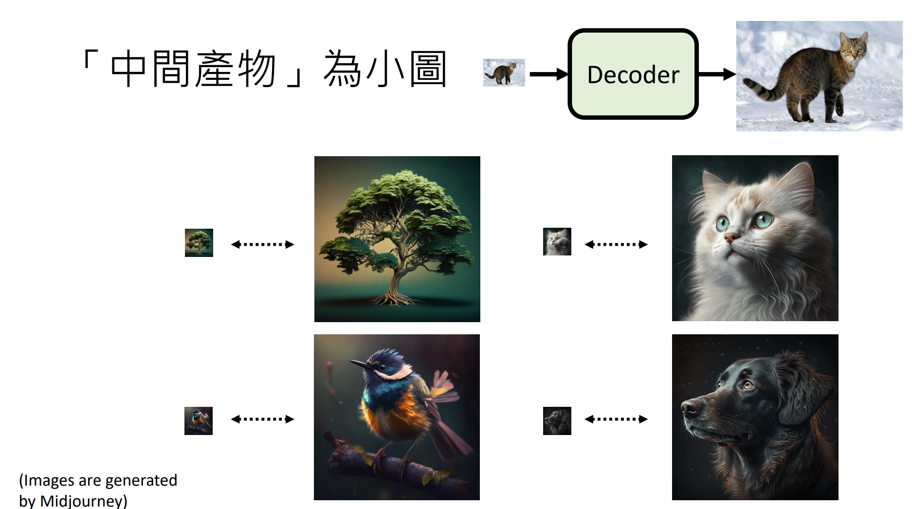
1. A smaller version of the original image (Imagen): we can train this decoder in a supervised learning manner.
2. Latent representation (Stable Diffusion, DALL-E): we can train this decoder via AE.

The following is the pipeline of stable diffusion, which is similar to the common architecture:

Fig. 9. Architecture of Stable Diffusion

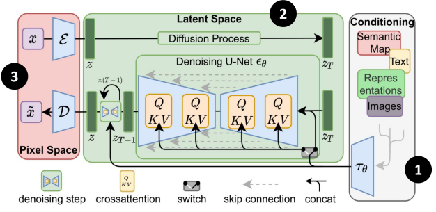
• In addition to text, stable diffusion also supports other conditional generation.
• Stable diffusion train decoder in latent space. Hence, while training, the training image is transformed to latent representation $z$ using the encoder of AE.
• The forward and denoising processes are also finished in the latent space.

Fig. 10. Forward in Latent Space

Why Diffusion Works

The diffusion model can actually be regarded as an autoregressive model with a global perspective. It ensures the integrity of the generated image while achieving self-correction through iterative denoising.